Here are the links to my previous articles on ML series
Part I
Part II
Part III
In this article, we will try to implement a simple linear regression example using Python. I am sure you are comfortable with Python, if not this is a good chance to learn Python while implementing ML algorithms. I will not explain the steps in detail as I have already done the same while implementing Linear Regression using Octave.
Simple Linear Regression Example (One Variable)
Here is the link to our dataset containing population and profit in different cities.
Here is a snapshot of our data
6.1101,17.592
5.5277,9.1302
8.5186,13.662
7.0032,11.854
5.8598,6.8233
8.3829,11.886
7.4764,4.3483
So we have a comma-separated dataset with Population (in 10,000s) in the first column and Profit ($ 10,000s) in the second column. Our first step should be to load this data into our program and try to visualize its contents. Here are the steps we will be performing to create our first ML algorithm using Linear Regression for one variable.
Algorithm Steps
Load data in variables
Visualize the data
Write a Cost function
Run Gradient descent for some iterations to come up with values of theta0 and theta1
Plot your hypothesis function to see if it crosses most of the data
Run predictions and see results
Python Implementation
1. Load data in variables
import numpy as np
import matplotlib.pyplot as plt
import pandas as pd

def LinearRegression():
    # Load CSV File in Variables
    data = pd.read_csv('franchisedata.txt',header = None)
Data will be loaded in a 2 x 2 matrix. Now we need to separate data into x and y variables. x being input, y output, and m being total examples in the dataset. You need to install numpy, matplotlib, and pandas using the pip3 command
import numpy as np
import matplotlib.pyplot as plt
import pandas as pd

def LinearRegression():
    # Load CSV File in Variables
    data = pd.read_csv('franchisedata.txt',header = None)

    # Transfer data in x & y variable
    x = np.array(data.iloc[:, :-1].values)
    y = np.array(data.iloc[:, -1].values)
    m = len(x)
2. Visualize the data
Let us visualize this data by plotting a graph.
import numpy as np
import matplotlib.pyplot as plt
import pandas as pd

def LinearRegression():
    # Load CSV File in Variables
    data = pd.read_csv('franchisedata.txt',header = None)

    # Transfer data in x & y variable
    x = np.array(data.iloc[:, :-1].values)
    y = np.array(data.iloc[:, -1].values)
    m = len(x)

    # Plot Data
    plt.scatter(x, y,marker='s',facecolors='none',edgecolors='b')
    plt.xlabel('Population of City in 10,000s')
    plt.ylabel('Profit in $10,000s')
    plt.show()
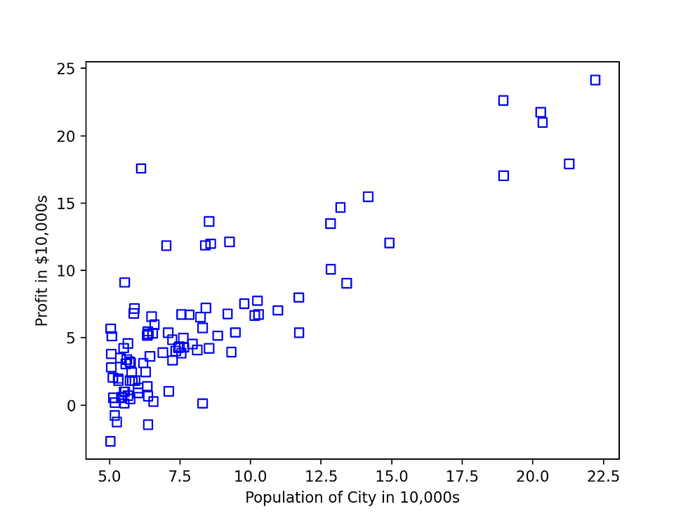
After running this code, the following graph will be displayed, you can run this code using the command python3 LinerRegression.py

Now we need to find a hypothesis function that will draw a straight line that will be best for our data.
3. Write a Cost function
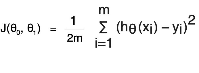
Our next task is to write a cost function so that we can use the same while performing Gradient descent and store the history of cost which can be used later. Before we calculate cost we need to first find h(θ).
h(θ) = theta0 + theta1 * x1;
We need to calculate the hypothesis for all values of x and sum it up to come up with a cost value for theta0 and theta1.

This can be done using a normal method or using a vectorized method where we will operate directly on the matrix. To understand better, let us first implement the cost function using the normal method. Also, remember that in Python matrix indices starts from 0
 # Calculate Cost using Normal method
 def CalculateCost(input, output, theta):
    m = len(output)
    cost = 0;
    for i in range(m):
        hypothesis = np.zeros(m)
        hypothesis[i] = theta[0] + theta[1]*input[i]
        cost = cost + (hypothesis[i] - output[i]) **2
        cost = cost/(2*m)
 return cost
our main function will look like this
def LinearRegression():
    # Load CSV File in Variables
    data = pd.read_csv('franchisedata.txt',header = None)

    # Transfer data in x & y variable
    x = np.array(data.iloc[:, :-1].values)
    y = np.array(data.iloc[:, -1].values)
    m = len(x)
    theta = np.array([0.00,0.00])

    # Plot Data
    plt.scatter(x, y,marker='s',facecolors='none',edgecolors='b')
    plt.xlabel('Population of City in 10,000s')
    plt.ylabel('Profit in $10,000s')
    plt.show()
    # Calculate Cost Using Theta as 0 defined above
    cost = CalculateCost(x,y,theta)
In order to calculate the cost using the vectorized method, we need to change our function a little bit
h(θ) = theta0*x0 + theta1 * x1;
Considering x0 =1, our above function will result in the same value as the original one. x0 is a new feature we added to our data set with the value 1. Let us modify our dataset
X = np.concatenate((np.ones((m,1), dtype=int), x), axis=1)This will add one more column to our input dataset x, now our input dataset will look like
X = [ 1 6.1101 1 5.5277 1 8.5186 1 7.0032 1 5.8598 1 8.3829 1 7.4764
]
Now calculating hypothesis is simple, just multiple X with the transpose of theta.
h(θ) = x * θ';
You can try out solving this equation in order to understand how this is calculating the values of the entire hypothesis matrix in one go. Our cost function will look like
 # Vectorized Implementation of Cost Function
 def CalculateCostVectorized(input, output, theta):
    m = len(output)
    cost = 0;
    hypothesis = np.zeros(m)
    hypothesis = input.dot(theta.T)
    cost = np.sum(np.subtract(hypothesis,output) **2)/(2*m)
    return cost
Let us modify the main function to call this cost function
def LinearRegression():
    # Load CSV File in Variables
    data = pd.read_csv('franchisedata.txt',header = None)

    # Transfer data in x & y variable
    x = np.array(data.iloc[:, :-1].values)
    y = np.array(data.iloc[:, -1].values)
    m = len(x)
    theta = np.array([0.00,0.00])

    # Plot Data
    plt.scatter(x, y,marker='s',facecolors='none',edgecolors='b')
    plt.xlabel('Population of City in 10,000s')
    plt.ylabel('Profit in $10,000s')
    plt.show()

    # Calculate Cost Using Theta as 0 defined above
    X = np.concatenate((np.ones((m,1), dtype=int), x), axis=1)
    cost = CalculateCostVectorized(X,y,theta)
4. Run Gradient Descent (GD)
To come up with the right values of theta0 and theta1 which provide minimum cost, we need to run a gradient descent algorithm for some number of iterations. Below is our gradient descent algorithm for calculating theta values

We need to start with some initial values of theta and alpha and run gradient descent. Let us consider our initial values as
    theta = np.array([0.00,0.00])
    alpha = 0.01
    iterations = 1500
Our GD function will look like below
 # Gradient Descent Function
 def runGradientDescent(input, output, theta, alpha, iterations):
    m = len(output)
    # Temp Variable
    t0 = 0.00
    t1 = 0.00

    for i in range(iterations):
        hypothesis = input.dot(theta.T)
        hypothesis = np.subtract(hypothesis,output)
        t0 = t0 - alpha*(1/m)* hypothesis.sum()
        t1 = t1 - alpha*(1/m)* (hypothesis * input[:,1]).sum()
        CalculateCostVectorized(input,output,theta)
        theta[0] = t0
        theta[1] = t1
    return theta
Running above GD function for 1500 iterations, theta comes out to be
theta = -3.6303 1.1664
5. Plot graph of Hypothesis function
Finally, we have received our theta values, let us calculate the hypothesis with these values and try to plot the hypothesis on our existing graph to see if it fits well on our data.
def LinearRegression():
    # Load CSV File in Variables
    data = pd.read_csv('franchisedata.txt',header = None)

    # Transfer data in x & y variable
    x = np.array(data.iloc[:, :-1].values)
    y = np.array(data.iloc[:, -1].values)
    m = len(x)
    theta = np.array([0.00,0.00])

    # Plot Data
    plt.scatter(x, y,marker='s',facecolors='none',edgecolors='b')
    plt.xlabel('Population of City in 10,000s')
    plt.ylabel('Profit in $10,000s')

    # Calculate Cost Using Theta as 0 defined above
    X = np.concatenate((np.ones((m,1), dtype=int), x), axis=1)
    cost = CalculateCostVectorized(X,y,theta)

    # Run GD
    alpha = 0.01
    iterations = 1500
    theta = runGradientDescent(X,y,theta,alpha, iterations)

    # Calculate Hypothesis & Plot Graph
    hypothesis = X.dot(theta)
    plt.plot(x,hypothesis,'r')
    plt.show()
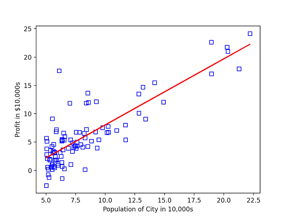
The following graph will be displayed

Looks like our function is able to converge with 1500 iterations. Practically you may need to run GD multiple times in order to see how it converges.
6. Run predictions & see results
Let us add one simple function to predict profit values with the population as input. Prediction is nothing but our hypothesis function with calculated values of theta.
 # Prediction based on Theta Values
 def predictProfit(input, theta):
    predition = theta[0] + theta[1] * input
 return predition
our main function will look like this
def LinearRegression():
    # Load CSV File in Variables
    data = pd.read_csv('franchisedata.txt',header = None)

    # Transfer data in x & y variable
    x = np.array(data.iloc[:, :-1].values)
    y = np.array(data.iloc[:, -1].values)
    m = len(x)
    theta = np.array([0.00,0.00])

    # Plot Data
    plt.scatter(x, y,marker='s',facecolors='none',edgecolors='b')
    plt.xlabel('Population of City in 10,000s')
    plt.ylabel('Profit in $10,000s')

    # Calculate Cost Using Theta as 0 defined above
    X = np.concatenate((np.ones((m,1), dtype=int), x), axis=1)
    cost = CalculateCostVectorized(X,y,theta)

    # Run GD
    alpha = 0.01
    iterations = 1500
    theta = runGradientDescent(X,y,theta,alpha, iterations)

    # Calculate hypothesis & Plot Graph
    hypothesis = X.dot(theta)
    plt.plot(x,hypothesis,'r')

    # Predictions
    population_one = 3.5;
    profit_one = predictProfit(population_one,theta);
    print(profit_one*10000)
    plt.plot(population_one,profit_one,'r',marker='s')

    population_two = 12;
    profit_two = predictProfit(population_two,theta);
    plt.plot(population_two,profit_two,'r',marker='s')
    print(profit_two*10000)
    plt.show()
Here is the entire source code of the above program
In my next article, I will provide details on how to implement Linear Regression for multiple input variables. This algorithm is also called Multivariant Linear Regression.
Happy Reading...
Comments