
Its time to dive deep into the Supervised Learning algorithm and find how to implement a Linear Regression function using multiple input parameters. If you arrived at this article directly, I would recommend you to have a look at previous posts from this series
Here are the links to my previous posts
Part I
Part II
Part III
Part IV
In my previous articles, we implemented a Linear Regression using Octave and Python. We covered an example where we have one input variable (population) and one output variable (profit).

Practically when we will implement ML solutions using LG, there is a very low probability that we have to deal with only one feature variable.
Data can have input features in 100s, 1000s, or even more. That's where you will be able to utilize the true potential of this algorithm.
For example, our profit calculator can have additional features like Average income, population, age, and many more. Let us see how to perform a supervised learning algorithm for multiple-input variables or features.
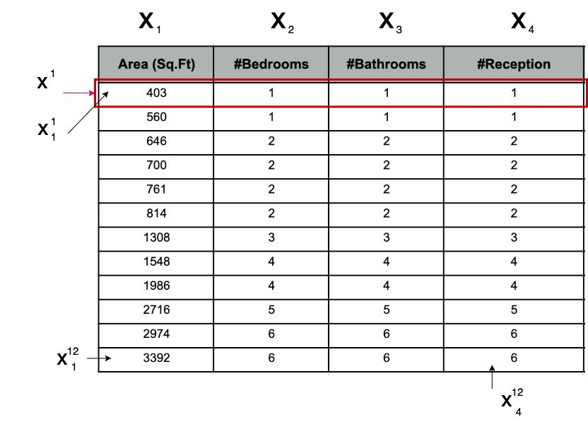
Here is a snapshot of the housing price data for the city of London
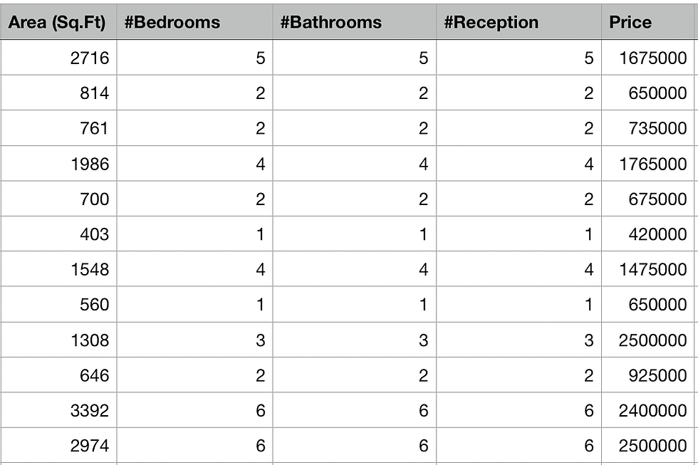
So now we have 4 features on which our housing price depends.
Feature Scaling
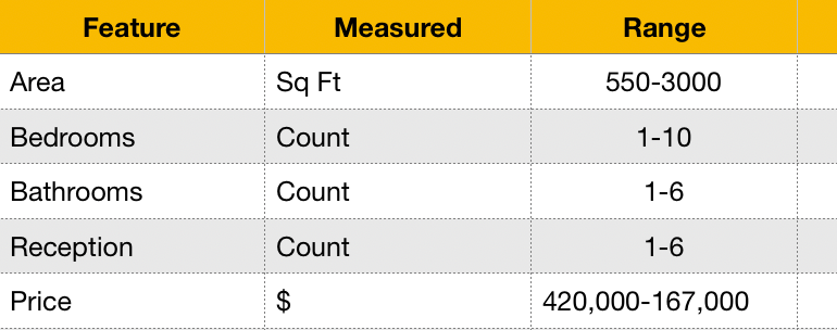
So we have 4 input features measured on a different scale altogether. One is in Sq.Ft ranges between 600 to 300 and others are counts ranges between 1-10 and output price in 10000s.
Consider a case where you have 100 or 1000 features with different scales. Now to run our hypothesis function and gradient descent functions on the feature of variant magnitudes, will not provide us desired results. Small features may not play any significant role in predictions. Also, gradient descent will take a much longer time to converge.
It is therefore very important to adjust different features to a similar scale and then run the algorithm.
Feature Scaling
Feature scaling is a preprocessing step used to normalize the range of data, it is also known as feature normalization. There are multiple ways in which you can scale your feature, one such is by performing a mathematical operation on your feature. If you recollect, we divided our housing price by 10,000. After obtaining the prediction results, we multiplied it by 10,000 to bring it back to the normal scale.
Ideally all our feature should be in the range of -1 <= x(i) <= 1 or -0.5 <= x(i) <= 0.5. In order to achieve such accurate results, we can use a mathematical technique called mean normalisation.
Min-Max Normalisation
Here is the formula for scaling a feature using Min-Max normalization.
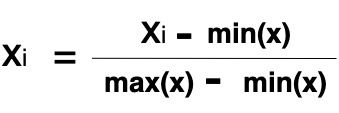
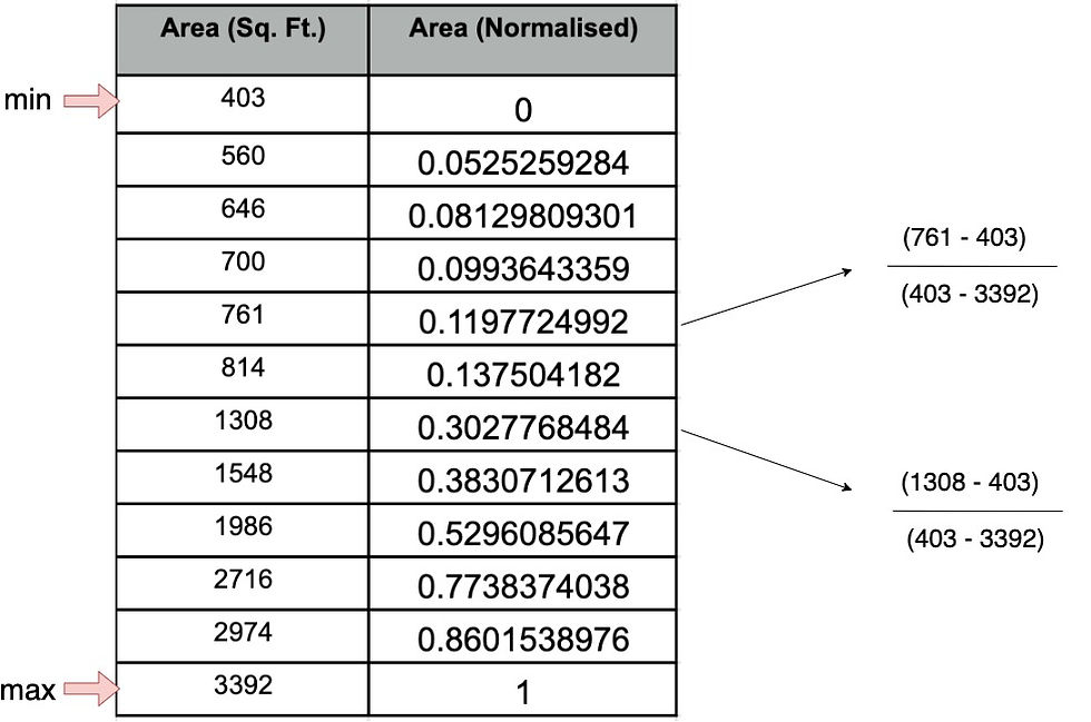
Let us try to normalize the features present in the above example, our final value will look like
Let us do the same for the number of bedrooms.
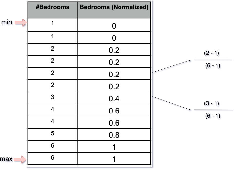
So how to come back to the original value once your prediction is complete? In the above case, you can use the formula
Area (Sq. Ft) = Normalized Area * (max-min) + min
for 2974 Area (Sq. Ft) .= 0.860153 * (3392 - 403) + 403 = 2974
Mean Normalization
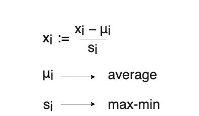
Another method of scaling your feature is the mean normalization method. Mean normalization is calculating by subtracting the average value from the original value and dividing the result by max-min value
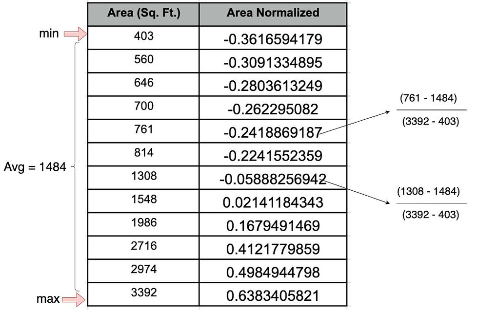
Let us try out mean normalization for the area
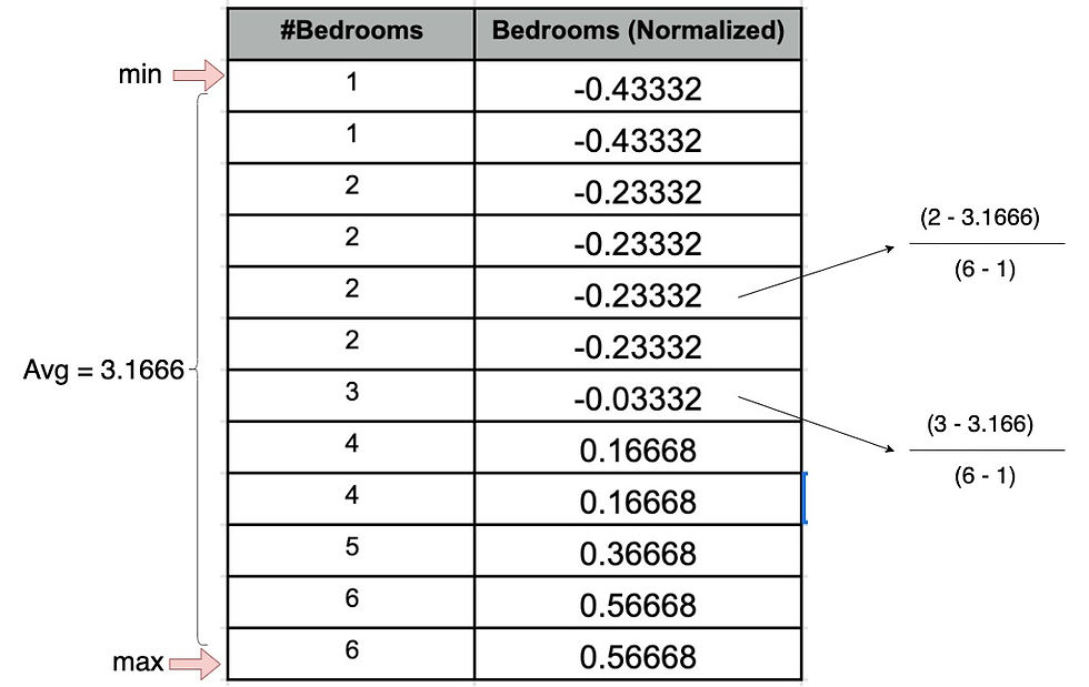
For the number of bedrooms
Let us try to calculate back our original value
Area (Sq. Ft) = Normalized Area * (max-min) + Average
for 2974 Area (Sq. Ft) .= 0.4984944798 * (3392 - 403) + 1484 = 2974
Now we know how to bring down your features at a similar scale it's time to come up with a hypothesis function and gradient function for multiple variable linear regression which is also called multivariate linear regression. Instead of using max-min you can also use standard deviation for the division. We have used the same in our practical examples.
Hypothesis & Gradient Descent
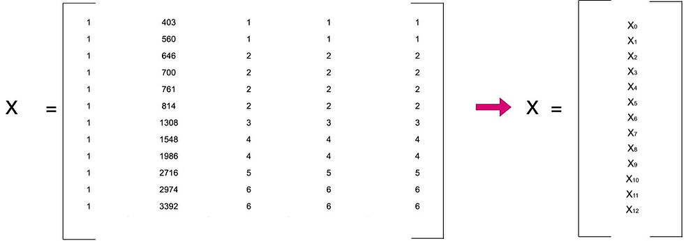
Let us try to visualize our data in matrix form.
X can be a two-dimensional metrics with 12 rows and 4 columns and Y will have 12 rows and 1 column

Remember how our hypothesis function looks like with one input feature?
In order to perform matrix multiplication, we added one additional feature X0 and our hypothesis looked like
and our vectorized implementation looks like
Let us add one more column to our input feature. It will look like this
The primary reason for using vectorized implementation was for after execution and also it is now very easy to implement the same algorithm for multiple features, let us find a hypothesis for multiple variables. For the above X & Y, our hypothesis function will be
Eventually
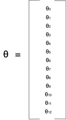
Where theta is
Gradient descent function will look like this
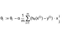
for j := 0...n
If you followed the last implementation of Gradient Descent and Hypothesis, using vectorized implementation for both will make the same code work with minor tweaks. I am sure you are pretty much eager to have a look at the implementation, we will implement this in our next article.
Here are a couple of more points that I would like to highlight which you should be aware of
Debugging Gradient Descent
So now we have implemented gradient descent to come up with optimal values of Thetas. How to debug the gradient descent algorithm and be assured it is working correctly?
When we run gradient descent, we initialize learning rate alpha and the number of iterations with some initial values. Running gradient descent is something that should be performed multiple times to adjust the learning rates and iterations suitable as per our need.
If you remember, in our last implementation of simple linear regression, while running gradient descent, we stored cost values during each iteration in an array. We can use this data to plot our cost against the number of iterations we are running. This will tell us if our gradient descent is taking us towards the minimal cost.
Consider below two graphs for the number of iterations and cost.
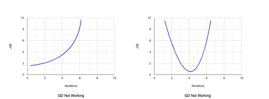
In the first graph, our cost is increasing with a number of iterations, surely GD is not working and we need to correct something. Usually, in such a case, we should use a smaller value of alpha. In the second graph or cost comes to a minimum value and increased again, clearly GD is not working and again we should be using a smaller value of Alpha.
Consider below graphs with much smaller values of learning rate alpha

In the first graph seems like cost is decreasing with iterations but not converged to a minimum, this means that we should increase the number of iterations.
In the second graph, we can see that cost decreased and then comes down to a minimum value and is not decreasing significantly with an increase in the number of iterations. That's where we can say that our gradient descent is converged to an optimum cost.
Features & Polynomial Regression
While selecting features, we can combine features to make our own features. For example, we can combine the Height & Width feature to come up with a new feature Area. We should also not use redundant features. For example, if we have an area in Sq. Ft. and also in Sq. Meters, we should select only one feature.
When we visualizing the data on an x, y-axis and if by looking at the data we realize that we can not fit a linear line within the data, it becomes imperative to change our linear function and make sure our prediction line fits the data well. In such a case, we can go for polynomial equations to come up with our hypothesis function.
Suppose we have a hypothesis function
We can create new features by using the same feature x, square(x), and cube(x), with these additional features our equation, will look like
I hope you all are following me very closely on these equations. There is an issue though with respect to overfitting your training examples if you are using high order polynomials or even if the number of features is high. We will see how to change our function to overcome the overfitting issue.
I my next article I will give an example that will implement Multivariate linear regression in Octave and possibly if time permits in Python.
Happy Reading....
Comments